
At Uber, real-time analytics allow us to attain business insights and operational efficiency, enabling us to make data-driven decisions to improve experiences on the Uber platform. For example, our operations team relies on data to monitor the market health and spot potential issues on our platform; software powered by machine learning models leverages data to predict rider supply and driver demand; and data scientists use data to improve machine learning models for better forecasting.
In the past, we have utilized many third-party database solutions for real-time analytics, but none were able to simultaneously address all of our functional, scalability, performance, cost, and operational requirements.
Released in November 2018, AresDB is an open source, real-time analytics engine that leverages an unconventional power source, graphics processing units (GPUs), to enable our analytics to grow at scale. An emerging tool for real-time analytics, GPU technology has advanced significantly over the years, making it a perfect fit for real-time computation and data processing in parallel.
In the following sections, we describe the design of AresDB and how this powerful solution for real-time analytics has allowed us to more performatively and efficiently unify, simplify, and improve Uber’s real-time analytics database solutions. After reading this article, we hope you try out AresDB for your own projects and find the tool useful your own analytics needs, too!
Real-time analytics applications at Uber
Data analytics are crucial to the success of Uber’s business. Among other functions, these analytics are used to:
- Build dashboards to monitor our business metrics
- Make automated decisions (such as trip pricing and fraud detection) based on aggregated metrics that we collect
- Make ad hoc queries to diagnose and troubleshoot business operations issues
We can summarize these functions into categories with different requirements as follows:
| Dashboards | Decision Systems | Ad hoc Queries | |
| Query Pattern | Well known | Well known | Arbitrary |
| Query QPS | High | High | Low |
| Query Latency | Low | Low | High |
| Dataset | Subset | Subset | All data |
Dashboards and decision systems leverage real-time analytical systems to make similar queries over relatively small, yet highly valuable, subsets of data (with maximum data freshness) at high QPS and low latency.
The need for another analytical engine
The most common problem that real-time analytics solves at Uber is how to compute time series aggregates, calculations that give us insight into the user experience so we can improve our services accordingly. With these computations, we can request metrics by specific dimensions (such as day, hour, city ID, and trip status) over a time range on arbitrarily filtered (or sometimes joined) data. Over the years, Uber has deployed multiple solutions to solve this problem in different ways.
Some of the third-party solutions we’ve used for solving this type of problem include:
- Apache Pinot, an open source distributed analytical database written in Java, can be leveraged for large-scale data analytics. Pinot employs a lambda architecture internally to query batch and real-time data in columnar storage, uses inverted bitmap index for filtering, and relies on star-tree for aggregate result caching. However, it does not support key-based deduplication, upsert, joins, and advanced query features such as geo-spatial-filtering. In addition, being a JVM-based database, query execution on Pinot runs at a higher cost in terms of memory usage.
- Elasticsearch is used at Uber for a variety of streaming analytics needs. It was built on Apache Lucene for full-text keyword search that stores documents and inverted index. It has been widely adopted and extended to also support aggregates. The inverted index enables filtering, yet it is not optimized for time range-based storage and filtering. It stores records as JSON documents, imposing additional storage and query access overhead. Like Pinot, Elasticsearch is a JVM-based database, and as such, does not support joins and its query execution runs at a higher memory cost.
While these technologies have strengths of their own, they lacked crucial functionalities for our use case. We needed a unified, simplified, and optimized solution, and thought outside-of-the-box (or rather, inside the GPU) to reach a solution.
Leveraging GPUs for real-time analytics
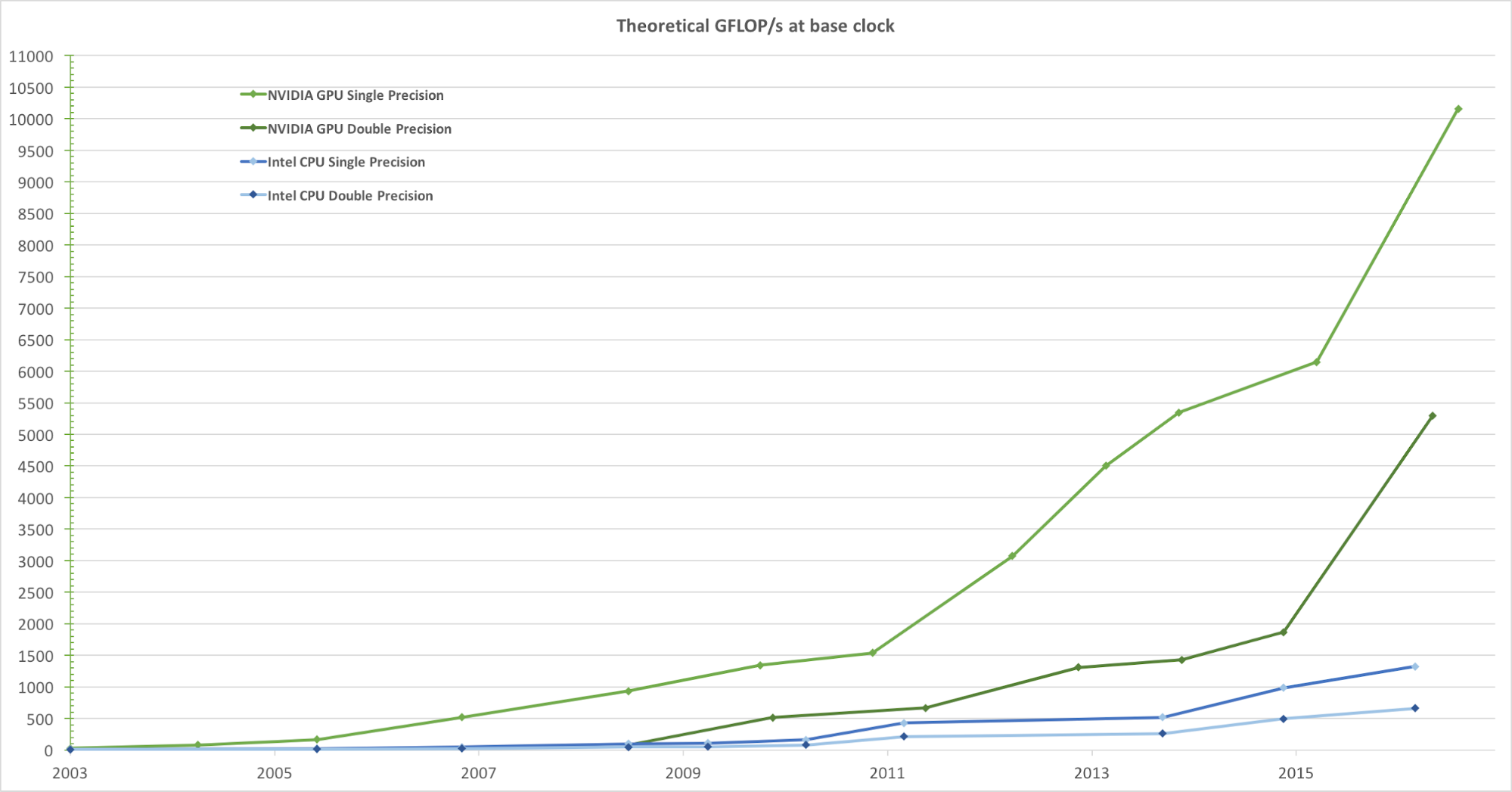
To render realistic views of images at a high frame rate, GPUs process a massive amount of geometries and pixels in parallel at high speed. While the clock-rate increase for processing units has plateaued over the past few years, the number of transistors on a chip has only increased per Moore’s law. As a result, GPU computation speeds, measured in Gigaflops per second (GFLOP/s), are rapidly increasing. Figure 1, below, depicts the theoretical GFLOP/s trend comparing NVIDIA GPUs and Intel CPUs over the years:
When designing our real-time analytics querying engine, integrating GPU processing was a natural fit. At Uber, the typical real-time analytical query processes a few days of data with millions to billions of records and then filters and aggregates them in a short amount of time. This computation task fits perfectly into the parallel processing model of general purpose GPUs because they:
- Process data in parallel very quickly.
- Deliver greater computation throughput (GFLOPS/s), making them a good fit for heavy computation tasks (per unit data) that can be parallelized.
- Offer greater compute-to-storage (ALU to GPU global memory) data access throughput (not latency) compared to central processing units (CPUs), making them ideal for processing I/O (memory)-bound parallel tasks that require a massive amount of data.
Once we settled on using a GPU-based analytical database, we assessed a few existing analytics solutions that leveraged GPUs for our needs:
- Kinetica, a GPU-based analytics engine, was initially marketed towards U.S. military and intelligence applications in 2009. While it demonstrates the great potential of GPU technology in analytics, we found many key features missing for our use case, including schema alteration, partial insertion or updates, data compression, column-level memory/disk retention configuration, and join by geospatial relationships.
- OmniSci, an open source, SQL-based query engine, seemed like a promising option, but as we evaluated the product, we realized that it did not have critical features for Uber’s use case, such as deduplication. While OminiSci open sourced their project in 2017, after some analysis of their C++-based solution, we concluded that neither contributing back nor forking their codebase was viable.
- GPU-based real-time analytics engines, including GPUQP, CoGaDB, GPUDB, Ocelot, OmniDB, and Virginian, are frequently used by academic institutions. However, given their academic purpose, these solutions focus on developing algorithms and designing proof of concepts as opposed to handling real-world production scenarios. For this reason, we discounted them for our scope and scale.
Overall, these engines demonstrate the great advantage and potential of data processing using GPU technology, and they inspired us to build our own GPU-based, real-time analytics solution tailored to Uber’s needs. With these concepts in mind, we built and open sourced AresDB.
AresDB architecture overview
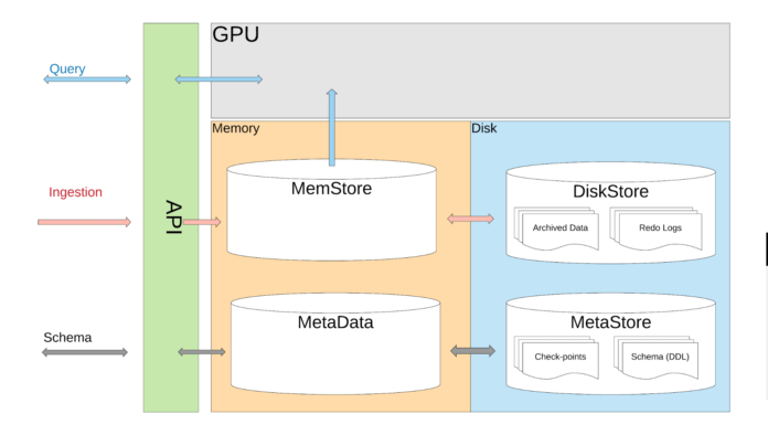
At a high level, AresDB stores most of its data in host memory (RAM that is connected to CPUs), handling data ingestion using CPUs and data recovery via disks. At query time, AresDB transfers data from host memory to GPU memory for parallel processing on GPU. As shown in Figure 2, below, AresDB consists of a memory store, a meta datastore, and a disk store:
Tables
Unlike most relational database management systems (RDBMSs), there is no database or schema scope in AresDB. All tables belong to the same scope in the same AresDB cluster/instance, enabling users to refer to them directly. Users store their data as fact tables and dimension tables.
Fact table
A fact table stores an infinite stream of time series events. Users use a fact table to store events/facts that are happening in real time, and each event is associated with an event time, with the table often queried by the event time. An example of the type of information stored by fact tables are trips, where each trip is an event and the trip request time is often designated as the event time. In case an event has multiple timestamps associated with it, only one timestamp is designated as the time of the event displayed in the fact table.
Dimension table
A dimension table stores current properties for entities (including cities, clients, and drivers). For example, users can store city information, such as city name, time zone, and country, in a dimension table. Compared to fact tables, which grow infinitely over time, dimension tables are always bounded by size (e.g., for Uber, the cities table is bounded by the actual number of cities in the world). Dimension tables do not need a special time column.
Data types
Table below details the current data types supported in AresDB:
| Data Types | Storage (in Bytes) | Details |
| Bool | 1/8 | Boolean type data, stored as single bit |
| Int8, Uint8 | 1 | Integer number types. User can choose based on cardinality of field and memory cost. |
| Int16, Uint16 | 2 | |
| Int32, Uint32 | 4 | |
| SmallEnum | 1 | Strings are auto translated into enums. SmallEnum can holds string type with cardinality up to 256 |
| BigEnum | 2 | Similar to SmallEnum, but holds higher cardinality up to 65535 |
| Float32 | 4 | Floating point number. We support Float32 and intend to add Float64 support as needed |
| UUID | 16 | Universally unique identifier |
| GeoPoint | 4 | Geographic points |
| GeoShape | Variable Length | Polygon or multi-polygons |
With AresDB, strings are converted to enumerated types (enums) automatically before they enter the database for better storage and query efficiency. This allows case-sensitive equality checking, but does not support advanced operations such as concatenation, substrings, globs, and regex matching. We intend to add full string support in the future.
Key features
AresDB’s architecture supports the following features:
- Column-based storage with compression for storage efficiency (less memory usage in terms of bytes to store data) and query efficiency (less data transfer from CPU memory to GPU memory during querying)
- Real-time upsert with primary key deduplication for high data accuracy and near real-time data freshness within seconds
- GPU powered query processing for highly parallelized data processing powered by GPU, rendering low query latency (sub-seconds to seconds)
Columnar storage
Vector
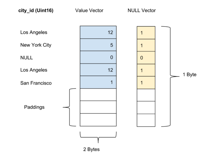
AresDB stores all data in a columnar format. The values of each column are stored as a columnar value vector. Validity/nullness of the values in each column is stored in a separate null vector, with the validity of each value represented by one bit.
Live store
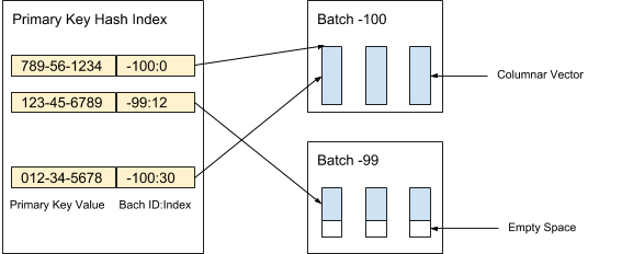
AresDB stores uncompressed and unsorted columnar data (live vectors) in a live store. Data records in a live store are partitioned into (live) batches of configured capacity. New batches are created at ingestion, while old batches are purged after records are archived. A primary key index is used to locate the records for deduplication and updates. Figure 3, below, demonstrates how we organize live records and use a primary key value to locate them:
The values of each column within a batch are stored as a columnar vector. Validity/nullness of the values in each value vector is stored as a separate null vector, with the validity of each value represented by one bit. In Figure 4, below, we offer an an example with five values for a city_id column:
Archive store
AresDB also stores mature, sorted, and compressed columnar data (archive vectors) in an archive store via fact tables. Records in archive store are also partitioned into batches. Unlike live batches, an archive batch contains records of a particular Universal Time Coordinated (UTC) day. Archive batch uses the number of days since Unix Epoch as its batch ID.
Records are kept sorted according to a user configured column sort order. As depicted in Figure 5, below, we sort by city_id column first, followed by a status column:

The goal of configuring the user-configured column sort order is to:
- Maximize compression effects by sorting low cardinality columns earlier. Maximized compression increases storage efficiency (less bytes needed for storing data) and query efficiency (less bytes transferred from CPU to GPU memory).
- Allow cheap range-based prefiltering for common equi-filters such as city_id=12. Prefiltering enables us to minimize the bytes needed to be transferred from CPU memory to GPU memory, thereby maximizing query efficiency.
A column is compressed only if it appears in the user-configured sort order. We do not attempt to compress high cardinality columns because the amount of storage saved by compressing high cardinality columns is negligible.
After sorting, the data for each qualified column is compressed using a variation of run-length encoding. In addition to the value vector and null vector, we introduce the count vector to represent a repetition of the same value.
Real-time ingestion with upsert support
Clients ingest data through the ingestion HTTP API by posting an upsert batch. The upsert batch is a custom, serialized binary format that minimizes space overhead while still keeping the data randomly accessible.
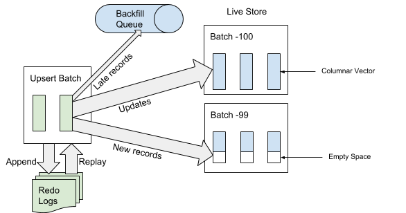
When AresDB receives an upsert batch for ingestion, it first writes the upsert batch to redo logs for recovery. After an upsert batch is appended to the end of the redo log, AresDB then identifies and skips late records on fact tables for ingestion into the live store. A record is considered “late” if its event time is older than the archived cut-off event time. For records not considered “late,” AresDB uses the primary key index to locate the batch within live store where they should be applied to. As depicted in Figure 6, below, brand new records (not seen before based on the primary key value) will be applied to the empty space while existing records will be updated directly:
Archiving
At ingestion time, records are either appended/updated in the live store or appended to a backfill queue waiting to be placed in the archive store.
We periodically run a scheduled process, referred to as archiving, on live store records to merge the new records (records that have never been archived before) into the archive store. Archiving will only process records in the live store with their event time falling into the range of the old cut-off time (the cut-off time from last archiving process) and new cut-off time (the new cut-off time based on the archive delay setting in the table schema).
The records’ times of event will be used to determine which archive batch the records should be merged into as we batch archived data into daily batches. Archiving does not require primary key value index deduplication during merging since only records between the old cut-off and new cut-off ranges will be archived.
Figure 7, below, depicts the timeline based on the given record’s event time:

In this scenario, the archiving interval is the time between two archiving runs, while the archiving delay is the duration after the event time but before an event can be archived. Both are defined in AresDB’s table schema configurations.
Backfill
As shown in Figure 7, above, old records (with event time older than the archiving cut-off) for fact tables are appended to the backfill queue and eventually handled by the backfill process. This process is also triggered by the time or size of the backfill queue onces it reaches its threshold. Compared to ingestion by the live store, backfilling is asynchronous and relatively more expensive in terms of CPU and memory resources. Backfill is used in the following scenarios:
- Handling occasional very late arrivals
- Manual fixing of historical data from upstream
- Populating historical data for recently added columns
Unlike archiving, backfilling is idempotent and requires primary key value-based deduplication. The data being backfilled will eventually be visible to queries.
The backfill queue is maintained in memory with a pre-configured size, and, during massive backfill loads, the client will be blocked from proceeding before the queue is cleared by a backfill run.
Query processing
With the current implementation, the user will need to use Ares Query Language (AQL), created by Uber to run queries against AresDB. AQL is an effective time series analytical query language and does not follow the standard SQL syntax of SELECT FROM WHERE GROUP BY like other SQL-like languages. Instead, AQL is specified in structured fields and can be carried with JSON, YAML, and Go objects. For instance, instead of SELECT count(*) FROM trips GROUP BY city_id WHERE status = ‘completed’ AND request_at >= 1512000000, the equivalent AQL in JSON is written as:
{
“table”: “trips”,
“dimensions”: [
{“sqlExpression”: “city_id”}
],
“measures”: [
{“sqlExpression”: “count(*)”}
],
“rowFilters”: [
“status = ‘completed'”
],
“timeFilter”: {
“column”: “request_at”,
“from”: “2 days ago”
}
}
In JSON-format, AQL provides better programmatic query experience than SQL for dashboard and decision system developers, because it allows them to easily compose and manipulate queries using code without worrying about issues like SQL injection. It serves as the universal query format on typical architectures from web browsers, front-end servers, and back-end servers, all the way back into the database (AresDB). In addition, AQL provides handy syntactic sugar for time filtering and bucketization, with native time zone support. The language also supports features like implicit sub-queries to avoid common query mistakes and makes query analysis and rewriting easy for back-end developers.
Despite the various benefits AQL provides, we are fully aware that most engineers are more familiar with SQL. Exposing a SQL interface for querying is one of the next steps that we will look into to enhance the AresDB user experience.
We depict the AQL query execution flow in Figure 8, below:
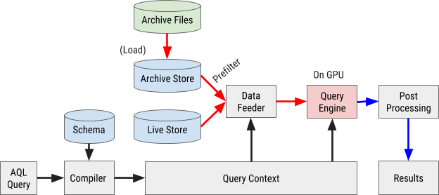
Query compilation
An AQL query is compiled into internal query context. Expressions in filters, dimensions, and measurements are parsed into abstract syntax trees (AST) for later processing via GPU.
Data feeding
AresDB utilizes pre-filters to cheaply filter archived data before sending them to a GPU for parallel processing. Since archived data is sorted according to a configured column order, some filters may be able to utilize this sorted order by applying binary search to locate the corresponding matching range. In particular, equi-filters on all of the first X-sorted columns and optionally range filter on sorted X+1 columns can be processed as pre-filters, as depicted in Figure 9, below:

After prefiltering, only the green values (satisfying filter condition) need to be pushed to the GPU for parallel processing. Input data is fed to the GPU and executed there one batch at a time. This includes both live batches and archive batches.
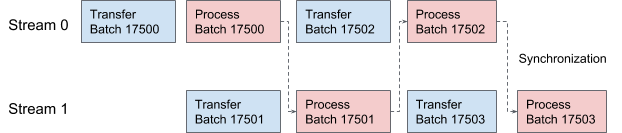
AresDB utilizes CUDA streams for pipelined data feeding and execution. Two streams are used alternately on each query for processing in two overlapping stages. In Figure 10, below, we offer a timeline illustration of this process:
Query execution
For simplicity, AresDB utilizes the Thrust library to implement query execution procedures, which offers fine-tuned parallel algorithm building blocks for quick implementation in the current query engine.
In Thrust, input and output vector data is accessed using random access iterators. Each GPU thread seeks the input iterators to its workload position, reads the values and performs the computation, and then writes the result to the corresponding position on the output iterator.
AresDB follows the one-operator-per-kernel (OOPK) model for evaluating expressions.
Figure 11, below, demonstrates this procedure on an example AST, generated from a dimension expression request_at – request_at % 86400 in the query compilation stage:
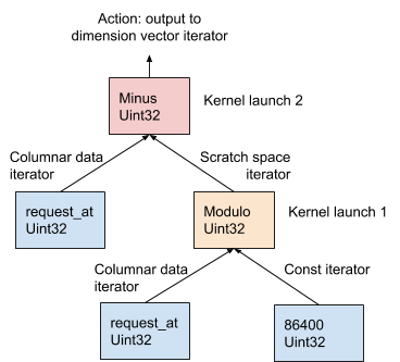
In the OOPK model, the AresDB query engine traverses each leaf node of the AST tree and returns an iterator for its parent node. In cases where the root node is also a leaf, the root action is taken directly on the input iterator.
At each non-root non-leaf node (modulo operation in this example), a temporary scratch space vector is allocated to store the intermediate result produced from request_at % 86400 expression. Leveraging Thrust, a kernel function is launched to compute the output for this operator on GPU. The results are stored in the scratch space iterator.
At the root node, a kernel function is launched in the same manner as a non-root, non-leaf node. Different output actions are taken based on the expression type, detailed below:
- Filter action to reduce the cardinality of input vectors
- Write dimension output to the dimension vector for later aggregation
- Write measure output to the measure vector for later aggregation
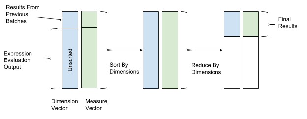
After expression evaluation, sorting and reduction are executed to conduct final aggregation. In both sorting and reduction operations, we use the values of the dimension vector as the key values of sorting and reduction, and the values of the measure vector as the values to aggregate on. In this way, rows with same dimension values will be grouped together and aggregated. Figure 12, below, depicts this sorting and reduction process:
AresDB also supports the following advanced query features:
- Join: currently AresDB supports hash join from fact table to dimension table
- Hyperloglog Cardinality Estimation: AresDB implements Hyperloglog algorithm
- Geo Intersect: currently AresDB supports only intersect operations between GeoPoint and GeoShape
Resource management
As an in-memory-based database, AresDB needs to manage the following types of memory usage:
| Allocation | Management Mode | |
| Live Store Vectors (live store columnar data) | C | Tracked |
| Archive Store Vectors (archive store columnar data) | C | Managed (Load and eviction) |
| Primary Key Index (hash table for record deduplication) | C | Tracked |
| Backfill Queue (store “late” arrival data waiting for backfill) | Golang | Tracked |
| Archive / Backfill Process Temporary Storage (Temporary memory allocated during the Archive and Backfill process) | C | Tracked |
| Ingestion / Query Temporary Storage;
Process Overheads; Allocation fragmentations |
Golang and C | Statically Configured Estimate |
When AresDB goes into production, it leverages a configured total memory budget. This budget is shared by all six memory types and should also leave enough room for the operating system and other processes. This budget also covers a statically configured overhead estimation, live data storage monitored by the server, and archived data that the server can decide to load and evict depending on the remaining memory budget.
Figure 13, below, depicts the AresDB host memory model:
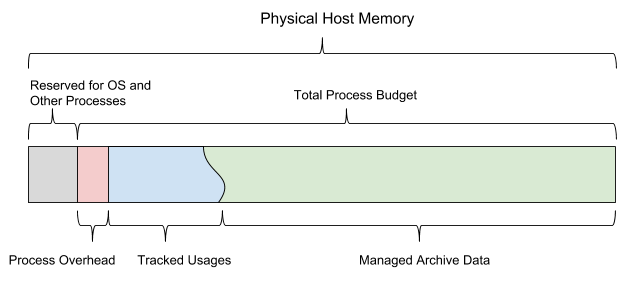
AresDB allows users to configure pre-loading days and priority at the column level for fact tables, and only pre-loads archive data within pre-loading days. Non-preloaded data is loaded into memory from disk on demand. Once full, AresDB also evicts archived data from the host memory. AresDB’s eviction policies are based on the number of preloading days, column priorities, the day of the batch, and the column size.
AresDB also manages multiple GPU devices and models device resources as GPU threads and device memory, tracking GPU memory usage as processing queries. AresDB manages GPU devices through device manager, which models GPU device resources in two dimensions–GPU threads and device memory–and tracks the usage while processing queries. After query compilation, AresDB enables users to estimate the amount of resources needed to execute the query. Device memory requirements must be satisfied before a query is allowed to start; the query must wait to run if there is not enough memory at that moment on any device. Currently, AresDB can run either one or several queries on the same GPU device simultaneously, so long as the device satisfies all resource requirements.
In the current implementation, AresDB does not cache input data in device memory for reuse across multiple queries. AresDB targets supporting queries on datasets that are constantly updated in real time and hard to cache correctly. We intend to implement a data caching functionality GPU memory in future iterations of AresDB, a step that will help optimize query performance.
Use Case: Uber’s Summary Dashboard
At Uber, we use AresDB to build dashboards for extracting real-time business insights. AresDB plays the role of storing fresh raw events with constant updates and computing crucial metrics against them in sub seconds using GPU power with low cost so that users can utilize the dashboards interactively. For example, anonymized trip data, which has a long lifespan in the datastore, is updated by multiple services, including our dispatch, payments, and ratings systems. To utilize trips data effectively, users will slice and dice the data into different dimensions to get insights for real-time decisions.
Leveraging AresDB, Uber’s Summary Dashboard is a widely used analytics dashboard leveraged by teams across the company to retrieve relevant product metrics and respond in real time to improve user experience.
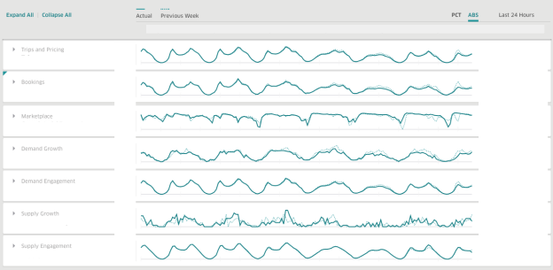
To build the mock-up dashboard, above, we modeled the following tables:
Trips (fact table)
| trip_id | request_at | city_id | status | driver_id | fare |
| 1 | 1542058870 | 1 | completed | 2 | 8.5 |
| 2 | 1541977200 | 1 | rejected | 3 | 10.75 |
| … |
Cities (dimension table)
| city_id | city_name | timezone |
| 1 | San Francisco | America/Los_Angeles |
| 2 | New York | America/New_York |
| … |
Table schemas in AresDB
To create the two modeled tables described above, we will first need to create the tables in AresDB in the following schemas:
| Trips | Cities |
| { “name”: “trips”, “columns”: [ { “name”: “request_at”, “type”: “Uint32”, }, { “name”: “trip_id”, “type”: “UUID” }, { “name”: “city_id”, “type”: “Uint16”, }, { “name”: “status”, “type”: “SmallEnum”, }, { “name”: “driver_id”, “type”: “UUID” }, { “name”: “fare”, “type”: “Float32”, } ], “primaryKeyColumns”: [ 1 ], “isFactTable”: true, “config”: { “batchSize”: 2097152, “archivingDelayMinutes”: 1440, “archivingIntervalMinutes”: 180, “recordRetentionInDays”: 30 }, “archivingSortColumns”: [2,3] } |
{ “name”: “cities”, “columns”: [ { “name”: “city_id”, “type”: “Uint16”, }, { “name”: “city_name”, “type”: “SmallEnum” }, { “name”: “timezone”, “type”: “SmallEnum”, } ], “primaryKeyColumns”: [ 0 ], “isFactTable”: false, “config”: { “batchSize”: 2097152 } } |
As described in schema, trips tables are created as fact tables, representing trips events that are happening in real time, while cities tables are created as dimension tables, storing information about actual cities.
After tables are created, users may leverage the AresDB client library to ingest data from an event bus such as Apache Kafka, or streaming or batch processing platforms such as Apache Flink or Apache Spark.
Sample queries against AresDB
In the mock-up dashboards, we choose two metrics as examples, total trip fare and active drivers. In the dashboard, users can filter the city for the metrics, eg. San Francisco. To draw the time series for these two metrics for the last 24 hours shown in the dashboards, we can run the following queries in AQL:
| Total trips fare in San Francisco in the last 24 hours group by hours | Active drivers in San Francisco in the last 24 hours group by hours |
| { “table”: “trips”, “joins”: [ { “alias”: “cities”, “name”: “cities”, “conditions”: [ “cities.id = trips.city_id” ] } ], “dimensions”: [ { “sqlExpression”: “request_at”, “timeBucketizer”: “hour” } ], “measures”: [ { “sqlExpression”: “sum(fare)” } ], “rowFilters”: [ “status = ‘completed'”, “cities.city_name = ‘San Francisco'” ], “timeFilter”: { “column”: “request_at”, “from”: “24 hours ago” }, “timezone”: “America/Los_Angeles” } |
{ “table”: “trips”, “joins”: [ { “alias”: “cities”, “name”: “cities”, “conditions”: [ “cities.id = trips.city_id” ] } ], “dimensions”: [ { “sqlExpression”: “request_at”, “timeBucketizer”: “hour” } ], “measures”: [ { “sqlExpression”: “countDistinctHLL(driver_id)” } ], “rowFilters”: [ “status = ‘completed'”, “cities.city_name = ‘San Francisco'” ], “timeFilter”: { “column”: “request_at”, “from”: “24 hours ago” }, “timezone”: “America/Los_Angeles” } |
Sample results from the query:
The above mock-up queries will produce results in the following time series result, which can be easily drawn into time-series graphs, as shown below:
| Total trips fare in San Francisco in the last 24 hours group by hours | Active drivers in San Francisco in the last 24 hours group by hours |
| { “results”: [ { “1547060400”: 1000.0, “1547064000”: 1000.0, “1547067600”: 1000.0, “1547071200”: 1000.0, “1547074800”: 1000.0, … } ] } |
{ “results”: [ { “1547060400”: 100, “1547064000”: 100, “1547067600”: 100, “1547071200”: 100, “1547074800”: 100, … } ] } |
In the above example, we demonstrated how to leverage AresDB to ingest raw events happening in real-time within seconds and issue arbitrary user queries against the data right away to compute metrics in sub seconds. AresDB helps engineers to easily build data products that extract metrics crucial to businesses that requires real-time insights for human or machine decisions.
Next steps
AresDB is widely used at Uber to power our real-time data analytics dashboards, enabling us to make data-driven decisions at scale about myriad aspects of our business. By open sourcing this tool, we hope others in the community can leverage AresDB for their own analytics.
In the future, we intend to enhance the project with the following features:
- Distributed design: We are working on building out the distributed design of AresDB, including replication, sharding management, and schema management to improve its scalability and reduce operational costs.
- Developer support and tooling: Since open sourcing AresDB in November 2018, we have been working on building more intuitive tooling, refactoring code structures, and enriching documentation to improve the onboarding experience, enabling developers to quickly integrate AresDB to their analytics stack.
- Expanding feature set: We also plan to expand our query feature set to include functionality such as window functions and nested loop joins, thereby allowing the tool to support more use cases.
- Query engine optimization: We will also be looking into developing more advanced ways to optimize query performance, such as Low Level Virtual Machine (LLVM) and GPU memory caching.
AresDB is open sourced under the Apache License. We encourage you to try out AresDB and join our community.
If building large-scale, real-time data analytics technologies interests you, consider applying for a role on our team.
Acknowledgements
Special thanks to Kate Zhang, Jennifer Anderson, Nikhil Joshi, Abhi Khune, Shengyue Ji, Chinmay Soman, Xiang Fu, David Chen, and Li Ning for making this project a fabulous success!